transformation – Globbering Mattress

A long time ago, I had animated the deck transformations of the covering space of a pair of circles. I’m talking about this blog post.

A lot of time has passed and I couldn’t help but rethink it in the light of some insights that I later had after the post. The deck transformations that I had created in my first attempt are quite unnatural. The reason is simply that a Cayley graph of a free group of two generators cannot be embedded inside ${\mathbb{R}^2}$ with the geometry intact. Therefore, any attempt to visualize the Cayley graph in that setting means forgetting about the geometry.

However, there is one setting in which the Cayley graph can naturally exist, without lying about its geometry. And that place is the hyperbolic 2-space (or hyperbolic n-space)! I was inspired by this idea when I found about this project called Walrus. This program is a way to visualize exponentially growing graphs using tools of hyperbolic geometry. The Cayley graph discussed in the previous blog post is also an exponentially growing graph.

Earlier, we had considered the universal covering space of the following topological space (think of it as a subspace of ${\mathbb{R}^2}$ ).

The covering space looked like the following. It is a graph, better expressed with a bunch of line segments quotiented away at the nodes that connect them.

Notice that the above graph is the same as the following graph. All the vertices are tetravalent like how they should be. As some of you may be able to guess, this graph is actually embedded inside the Poincare disc, with the line segments now being the Hyperbolic geodesics of the negative curvature space.

For clearer understanding, let us glance over what I mean. As a set, the Poincare disc ${D}$ is given by

$\displaystyle D= \{ z \in \mathbb{C} \ | \ |z| < 1\}. \ \ \ \ \ (1)$

However, I would be kidding you if I told you that this is it. The Poincare disc is a metric space with the following metric. For two points ${z_1,z_2 \in D}$ , the distance ${d(z_1,z_2)}$ between them is given by

$\displaystyle \cosh(d(z_1,z_2)) = 1 + 2\frac{|z_1-z_2|^2}{(1-|z_1|^2)(1-|z_2|^2)} . \ \ \ \ \ (2)$

Of course, this bizarre formula is not very telling. It’s not even clear why this is a metric (for instance, why does it satisfy the triangle inequality?). Questions like these, and why this metric space is interesting will require a lot of discussion and we’ll not get into it. Interested readers can find this in plenty of books. To get a short introduction, you can watch this numberphile video.

The group of isometries (set of distance preserving homeomorphisms ${D \rightarrow D}$ ) of the space ${D}$ also happen to have a very neat and natural description. It is the group ${PSU(1,1)}$ which is the group defined as

$\displaystyle PSU(1,1):= \{ \left( \substack{a\ b \\ \bar{b}\ \bar{a}} \right)\ ,|a|^2-|b|^2=1 , (a,b,c,d) \in \mathbb{C}^4 \} / \{ \pm 1\} . \ \ \ \ \ (3)$

The action of this group on ${D}$ is via

$\displaystyle z \mapsto \frac{az+b}{cz+d}. \ \ \ \ \ (4)$

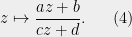
Enthusiastic readers of my blog (if there are any) will be able to relate the above formula to the modular group action in this blog post. They’re both examples of fractional linear transformations. In fact, the group ${PSU(1,1)}$ is isomorphic to the group ${PSL(2,\mathbb{C})}$ via a conjugation by some matrix (there are many such). Talking about this will lead us to the upper-half plane model of Hyperbolic geometry, the discussion of which we will save for some other time.

I am interested in two particular matrices:

$\displaystyle A:= \pm \Big{(} \substack{\sqrt{2}\ \ 1 \\ 1 \ \ \sqrt{2}}\Big{)} ,\ B:= \pm \Big{(} \substack{\sqrt{2}\ \ i \\ -i\ \ \sqrt{2}} \Big{)}. \ \ \ \ \ (5)$

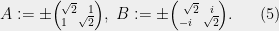
These matrices are carefully chosen, so that the following happens. Here is the action of ${A}$ on the picture produced previously.

Here is the action of ${B}$ .

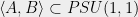
How were those specific matrices calculated? It’s enough for me to show this picture to you perhaps. This is the fundamental region of the group ${\langle A,B \rangle \subset PSU(1,1)}$ , which is the subgroup of ${PSU(1,1)}$ generated by the matrices ${A}$ and ${B}$ .Generating the entire tiling using the above fundamental region gives us the following pictures (the pointy edges in the four corners are something that is unnatural. It is because I could only calculate finitely many tiles. Those pointy corners would look denser, if it were calculated by a computer that had more time).

Here are the actions of ${A}$ and ${B}$ on the above picture.

For clarity, I will also demonstrate the Cayley tree with the tiling appearing faintly in the background.

This group ${\langle A, B\rangle}$ is, in fact, isomorphic to the free group of two generators, as you would expect. It must be isomorphic to the group of deck transformations of the covering space of ${B}$ . Another direct way to prove it is to use the Ping-Pong lemma.

Here are some more trippy visuals of the action of ${A}$ and ${B}$ .

Although in the previous post I had made a visualization of the covering map itself, I don’t think there is a natural way that map can be visualized using hyperbolic isometries, without which the purity of the Hyperbolic space will be ruined. If any of my readers gets an insight of having a way to map the Cayley tree to the wedge of two circles in a natural way, I would be excited to listen to your opinions in the comments.

One important discussion here may be the fact that ${\frac{D}{\langle A, B\rangle}}$ , which is the topological space of orbits of ${D}$ under the action of ${\langle A, B\rangle}$ , is homeomorphic to a torus with a point removed. A torus with a point removed has the same homotopy equivalence (and hence the same fundamental group) as that of a wedge of two circles (How? I wouldn’t ruin it for you). Do you smell a connection? It’s an interesting bedtime thought, trying to put this picture together. Someday maybe in a future project, I will try to make a visualization about it.

Here’s an exercise for you. Can you guess which element of ${\langle A, B\rangle}$ does the following transformation correspond to?

This blog post will be about the following animation, that I had created a while ago. Through this blog post, I will try to explain what I am trying to explain in the given visual (due to the large size of the GIF, it may take some time for it to load completely on your web-browser). Here is the topic in hand:

There are several pieces of information that are being conveyed here. I will go through them individually. I will assume that the reader is familiar with basic topology.

Bethe lattice

What we are considering here is the Bethe Lattice of coordination number 4. A Bethe Lattice is a particular type of Cayley Graph, and the case that we are considering is, in fact, the most clearly given example on Wikipedia.

The Cayley graph of the free group on two generators a and b (picture from Wikipedia). Although the graph pictured below looks finite, the picture represents a tree with infinitely many nodes, built recursively from a chosen root.

cayley_graph_of_f2

For our purpose, we want to consider this infinite graph as a topological space. We will consider the topology for this Cayley graph as if it is a Simplicial 2-Complex, or to simply put, we will imagine this graph to be infinitely many line segments glued togeather at common vertices.

I will denote this topological space by $C$ .

Wedge of two circles

The wedge of two circles, or the rose with two petals, or the figure-8 space is the just the subset of $\mathbb{R}^2$ given by any pair of circles sharing exactly one point. The topology on this set, of course, is the induced topology. Here is a picture below for the sake of clarity.

I will call this topological space $B$ .

Covering map, covering space

For a topological space $X$ , a covering space of $X$ is a topological space $E$ coupled with a continous map $p:E \rightarrow X$ such that every $x \in X$ has a neighbourhood $U_x$ around $x$ such that $p^{-1}(U_x)$ is a collection of disjoint open sets $\cup_{\lambda \in \Lambda}U_\lambda$ and each one of those open sets $U_\lambda$ is homeomorphic to $U_x$ , the homeomorphism being $p|_{U_\lambda}$ . The map $p:E \rightarrow X$ is called a covering map.

The definition may appear more intuitive if one imagines it this way: A continuous map $p:E \rightarrow X$ is a covering map if each $x \in X$ has an “evenly covered” neighbourhood! And what is “evenly covered”? It means that there the neighbourhood is such that the inverse image of that neighbourhood is just disjoint homeomorphic copies of the neighbourhood, and the homeomorphism is actually via the map $p$ . One can find images and examples on Wikipedia to get more intuition about this definition.

Now consider our figure-8 space $B$ and our Cayley graph $C$ . We define a continuous map $q:C \rightarrow B$ in the following way. Map each of the tetravalent nodes of the Cayley graph to the centre and the attached edges to the appropriate circle.

The rendition of this map $q$ via a movement of the each point to its image is presented below.

Now looking at the above picture, it is a matter of concern to know if the map is truly continuous, as the smaller edges appear to be stretching too much. Indeed, this would not be the case if the Cayley graph is given the subspace topology of $\mathbb{R}^2$ . In such a scenario, our map will fail to be continuous (I will leave it to the reader to verify this claim formally). Since the topology considered is that of a Simplicial 2-complex, the map $q$ can be constructed by glueing togeather continuous maps on each edge.

And as a matter of fact, we get more! The map $q:C \rightarrow B$ is a covering map. This can be readily verified.

Deck transformations

We said that if we have a covering map $p:E \rightarrow X$ , then each $x \in X$ has a “evenly covered” neighbourhood. We can think of the preimage of this “evenly covered” neighbourhood as a deck of cards. Informally speaking, a homeomorphism of $E$ that shuffles this deck around is called a deck transformation.

Formally, a deck transformation is a homeomorphism $f:E \rightarrow E$ of the covering space such that $p\circ f = p$ .

Clearly, such a map will have to permute all the preimages of any point in $X$ via $p$ . For our very own covering map $q:C \rightarrow B$ , we have the following two good deck transformations, again animated via a homotopy like the animation above.

In the image below, every tetravalent vertex on the main horizontal is mapped to the tetravalent vertex to its left. The animation runs the associated homotopy on an infinite loop.

hori1

Similar to the above image, each tetravalent vertex on the main vertical is mapped to the tetravalent vertex below it.

vert

Seeing the two maps inspires to compose the two maps and get a more visually pleasing homeomorphism. Please forgive my skills for the unpleasant abruptness in the animation.

Composing the horizontal and vertical displacements (the first two images) and their inverses can give us many deck transformations of the covering space $C$ . In fact, a little more investigation would reveal that these are all the deck transformations. However, that investigation will take up a lot of explanation. An interested reader can find everything relevant in a book like Hatcher’s Algebraic Topology.

What was that visual we started with?

With the visual that was given in the beginning, I attempted to illustrate the $p\circ f = p$ property of the horizontal deck transformation of the covering space $E$ . The animation unloads the covering space from the image, applies the deck transformation and applies the covering map again. Therefore in the animation above, we can actually see the shuffling of preimages.

—

With this, I mark the end of this blog post. If you are able to spot any mistakes, please comment below to inform me about it. If you think some points need to be explained more clearly, comment below. If you have any opinions, remarks, criticisms, please write them below. Most of all, if you have any ideas for making an animation about something sufficiently mathematical, do communicate about it below!

Aside: Although not so useful a terminology topologically speaking, the term “Kissing circles” is sometimes used for two circles sharing a tangential point. This term was perhaps poetically introduced by Frederick Soddy in the context of Descartes’ theorem. You can find his piece of trigonometric romance here.

Tag: transformation

A pair of circles sitting under a tree, K I S S I N G!